The G7 Main Window and Some Basic G7 Commands
The G7 Main Window is shown below, and consists of a menu bar, a button bar, a command box for typing commands, and an output window. At any time, you may click Help, or the little book button on the button bar, and read an online tutorial on using G7.
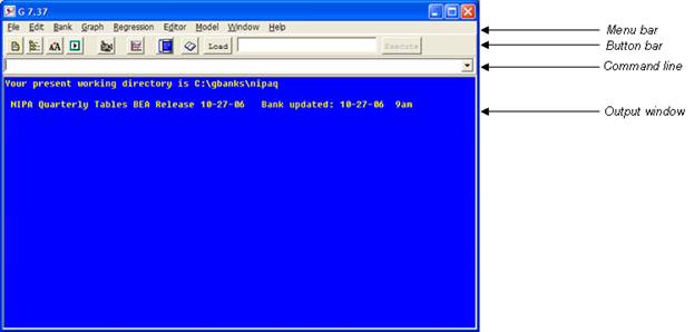
The G7 Main Window
Many of the features of G7 can be used either from the menu or from the command box. Where this is the case, we will show both methods. However, the real power of G7 comes from its command language which can be used to build programs or scripts, called add files, that automate data manipulation and regression.
To use the command box, click the pointer in the white box. The first command we will use is called look, which shows the contents of the currently assigned G bank.
Type “look” in the command box, and then hit the [Enter] key. If you want to use the menu, then choose the menu option Bank | Look. A small dialog window will open with a list of the currently-assigned banks. Only one bank initially is assigned, which is nipaq. Click on nipaq, and click OK. This is equivalent to giving the look command from the command line.
A window like the one shown below will appear. This look window provides a convenient way to navigate through the databank and look at graphs and printouts of the NIPA quarterly time series. The window is showing the contents of a G7 stub file. The stub file simply is a text file. Comment lines in this file begin with a semicolon (‘;’). Lines with time series have the name of the series to the left of the semicolon and descriptive text to the right of the semicolon. You can scroll through the stub file in the look window by using the [PgUp] and [PgDn] keys, the arrow keys, or the scroll bars. You can also use the Find command to search for text in the stub file.
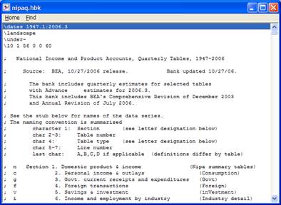
The Look Window
Use the Find command to find the series name “n01n01”. This is the G7 series name for Gross Domestic Product in the NIPA bank. The data are found in NIPA table 1.1.5, as shown below.
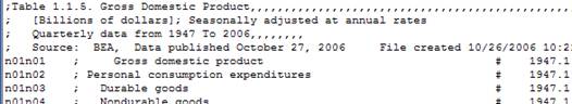
A NIPA Table
Now double-click on the line for Gross Domestic Product. In the G7 output window you will see a printout of the values of n01n01 (GDP) for the values of the current dates for printing. You can scroll back through the G7 output window using the scroll bar. If needed, text in that window can be selected and copied to the clipboard for pasting into other applications. A graph window (shown below) also will appear, showing a graph of the series for the current graph date interval.
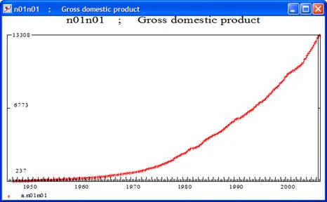
A Graph of GDP
You can resize the graph as you would any normal window. You can print the graph, in either landscape (full page) or portrait (half-page) mode, by picking Graph | Print. You can save the graph (in Windows metafile format, or *.WMF) so that you can include it in another document by selecting the menu item Graph | Save and then giving a file name.
Now, click in the command box again. Type the following command in the box, and hit the [Enter key]:
ty n01n01
You should see the same display in the output window that you got from double-clicking on the series line in the look window.
Now, graph the series manually by typing:
gr n01n01
You may see in the look window (if it still is open) that the series n01n02 is identified as Personal Consumption Expenditures. We will make a new graph of GDP and Personal Consumption, this time giving our own title. Type the lines below in the command box, each time hitting [Enter] at the end of the line:
ti GDP and Personal Consumption
gr n01n01 n01n02
You now should see the line for consumption appear in blue below the line for GDP. The title command (abbreviated ti) is for supplying a title for the graph. This graph is very busy, showing quarterly data for a fairly long period. Perhaps you would like to graph the series for a shorter interval. To graph the same series from the first quarter of 1990 to the third quarter of 2011, give the command:
gr n01n01 n01n02 1990.1 2011.3
This now will be the default starting and ending date for other graphs we make in G7. We can change the dates of the ty command in the same way:
ty n01n02 1995.1 2011.3
As with the graph dates, these dates will be remembered for the next ty command. In case you were wondering if you could set these dates up front, you can. Set the graph dates using the gdates command, and specify the type dates using the tdates command. For example, the following lines would set the same dates we had used in the above commands:
gdates 1990.1 2011.3
tdates 1995.1 2011.3
The series names that Inforum has developed for the NIPA bank are logical and correspond directly to table and line numbers in the NIPA. However, they are hard to remember. You can create a copy of a series in the bank in the G7 workspace bank by using the f (form) command. For example, we can make copies of GDP, Personal Consumption, and Gross Private Fixed Investment in the workspace bank, and then graph them, with the following commands:
f gdp = n01n01
f pce = n01n02
f gpfi = n01n06
ti GDP, PCE and GPFI
gr gdp pce gpfi
Another way of viewing the data is in grid format with the gridty (grid type) command. Give the following command and you will see a small spreadsheet window appear:
gridty gdp pce gpfi
This grid will display data for the current tdates setting.
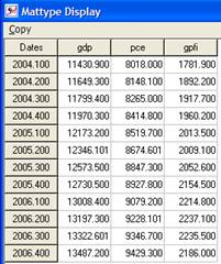
The GridType Window
If you would like to copy data from the grid to an Excel spreadsheet or to another application, scroll to the bottom right of the grid window and click in the lower, rightmost cell. Then click the Copy menu item at the top of the window. The following dialog will appear:
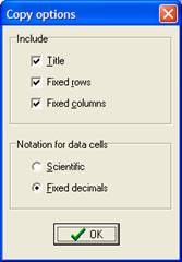
GridType Copy Options
The “Title”, “Fixed rows”, and “Fixed columns” check boxes allow you to specify if you would like the row and column headers (you probably do) and the title of the bank in your clipboard copy. The “Notation for data cells” choices allows you to copy the data either in scientific notation or with a fixed number of decimals. Now, open an Excel or OpenOffice Calc window and choose Edit | Paste, or Ctrl-V. The data from the G7 grid window now will be in your spreadsheet.
These are some introductory commands that enable you to browse the contents of a databank, print and graph timeseries data, and display and copy data in a spreadsheet format. We will explore some more G7 commands in a minute. First we will discuss the G7 command box in more depth, together with the button bar that appears just above the command box.