Running a Model - Deterministic Simulation

When a model has been built, the next step naturally is to run it, that is, to make simulations or forecasts with it. This is accomplished by selecting Model | Run. You will be presented with the form shown below.

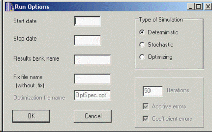
Macro Model Run Window

You first should select the type of simulation you wish to make in the panel in the top right. Most simulations or runs are deterministic, and we will initially assume that to be the case. The other two types of simulation are covered in the following two help topics.

Fill in the starting and stopping dates of the run. They should be in the usual form for dates in G7: 1980 for the year 1980, 1980.1 for the first quarter of 1980, and 1980.001 for January 1980.

Then fill in the name of the output bank. If you are running a historical simulation, HISTSIM would be a natural name. For a base forecast, BASE would be a good name; for high monetary growth scenario, HIMONEY could be a good name. This will be the root name of the .BNK and .IND files that compose the G7 data bank containing the results of the simulation.

Next, fill in the root name of the “fix” file. This is the file (which should have a file name without spaces and ending in .FIX) that provides values of exogenous variables with the (up)date commands and may in various ways to override or modify the results of the regression equations. The commands for doing so are rho, cta, mul, ovr, or skip.

To specify the complete course of the exogenous variable gR from 1995.1 to 2000.4, the command would be

update gR
1995.1 1411 1415 1413 1401
1996.1 1421 1429 1416 1419
1997.1 1435 1457 1462 1465
1998.1 1458 1483 1486 1494
1999.1 1512 1522 1544 1579
2000.1 1589 1610 1601 1617

Each line of the data begins with a date followed by the value of the variable in that quarter and as many successive value of the variable as you care to put on the line. Thus, this data could equally well have been supplied in the form

update gR
1995.1 1411 1415 1413 1401 1421 1429 1416 1419
1997.1 1435 1457 1997.3 1462 1465 1458 1483 1486 1494 1512 1522 1544
1999.9 1579 1589 1610 1601 1617

For specifying future values of an exogenous variable, it often is adequate to use linear interpolation between a small number of given values. A 0 in the data for an (up)date command means that the value is to be computed by linear interpolation. For example, the lines

update gR
2001.1 1630 0 0 0
2002.1 0 0 0 1700 0 0 0 0 0 0 0 0 0 0 0 1800

will make gR rise in a straight line from 1630 in 2001.1 to 1700 in 2002.4 and then on up by another straight line to 1800 in 2005.4.

The update command may be abbreviated as up. In counterhistorical simulations, that is, simulations over the historical period with some exogenous variables having values different than their historical values, it often is convenient to use the capacity of the update command to add a constant to all values of the variable or to multiply all values by a constant. Thus,

update gR +100

would add 100 to all values of gR, while

update gR -100

would subtract 100 from all values and

update gR *1.05

would multiply all values by 1.05.

You also can modify the values produced by the equations of the model. You could ask, for example, how the economy would have behaved if investment had always been 20 percent above what the equation predicted. Such modifications of the predicted values are referred to, somewhat disparagingly as “fixes.” There are five types of fixes available to you:

cta

Constant Term Adjustment fix (also called “adds”). Add a specified amount to the value calculated by the equation. The amount added can be different in different periods.

mul

Multiplicative fix. Multiply the value calculated from the equation by a specified factor, which may be different in different periods.

ovr

Override fix. Over-ride the equation. Discard the value calculated and use the one specified.

rho

Rho-adjustment fix. Add a rho-adjustment to the variable

skip

Skip fix. Ignore the value predicted by the equation and uses the historical value in its place.

The format for the first three is similar that of the (up)date command:

fixtype <variable_name>

<data lines>

For example,

cta cpcR
   1998.3 -20 -20 -25 -30 -30 -25 -15 -12 -10 -8 -4 -2 ;

The format for the rho-adjustment fix is

rho <variable_name> <rho_value>

For example,

rho vfR 0.9

The error of the regression equation in the starting year of the run will be calculated and then rho times this error will be added to the predicted value one period ahead, rho squared times the value added to the predicted value two periods ahead, and so on.

The format for skip is just

skip <variable_name>

For example,

skip cpcR

These fixes work only when applied to variables that are the dependent variable in a regression. When applied to other variables, the forecasting program does not reject them; it just never uses them. Furthermore, only one can be applied to any one variable. If more than one is applied, only the last takes effect. For example, if somewhere in the fix file after the above “cta cpcR” there should appear “rho CPCR 0.9”, the cta will be forgotten completely by the program without any warning.

When you click the OK button, a command prompt screen opens and you get a ] prompt. You may give any of the above commands at this point. Generally, however, you will have all of these commands in the .FIX file and will only wish to give a full title to your run, something like

ti Historical Simulation

You get the ] prompt again, and you type “run”, and the model runs. More precisely, when the OK button is clicked, a file by the name of _GO.BAT is created, a command prompt session is started, and this file executed. The folder that contains the model should also contain the file RUN.CFG, which may be copied from that for the AMI demonstration model.